Incunable leaf sizes

Confirmed: The earliest printed books look very much like books. Specifically, the ratio of leaf height to leaf width and the height-width ratio of the type space are precisely what you would expect.

That sounds complete uninteresting, but before making that statement in an article I'm working on, I wanted some actual data. That's the tricky part, however, as most incunable catalogs, and all of the incunable databases that I'm aware of, only record the format - as opposed to manuscript catalogs, which usually record the page dimensions, but not the format. Thanks to a tip from Oliver Duntze, I checked the British Museum incunable catalog. For 23 Mainz codex editions to 1470 recorded in BMC, the average leaf size ratio is 1: 1.44, while the type space ratio (from 25 editions) is a bit narrower, 1: 1.51. There is some variation, but most of these early printed books fall quite close to the mean, as the plot below shows. Leaf size is in red, while type space dimensions are in blue, with linear trend lines added to each.

 Fig. 1: Leaf height and width (red) and writing space height and width (blue) in Mainz codex editions to 1470.

To compare incunable leaf sizes rather than ratios, the BMC records for Mainz printing to 1470 might not be the best source, as many of those volumes are deluxe folio editions on vellum. Instead I referred to the Bodleian Library incunable catalog, which also provides leaf sizes. The graph below shows the leaf height for 15 folio editions, 26 quarto editions, and 2 octavo editions. More editions would of course be preferable, but since I don't have electronic records to work with, the data have to be entered manually. You can in any case already see the distinct formats: octavo leaf heights appear in red, quartos in gray, and folios in blue.

 Fig. 2: Leaf heights (mm) of a selection of folio (blue), quarto (gray), and octavo (red) incunables from the Bodleian Library.

Two things stand out: First, the folios clearly comprise different paper sizes, one with an average height around 290 mm, and another with an average height around 410 mm. Second, small quartos overlap with octavos. It would be interesting to look at more leaf sizes of these smaller formats.

The history of the late medieval book in one boxplot

One of the basic ways to describe the types used for fifteenth-century printed books is the method refined by Konrad Haebler that involves, among other things, measuring the height of twenty lines of type. The height of a typeface affected its legibility, or how far a reader could be from a text and still be able to read it. The height of the type was also significant in relation to the other types used in a book, as a type taller than the one used for the main text often identified titles and other structural paratexts, while a shorter type was typically used for marginal commentary. So what at first glance might sound like a number only interesting to antiquarians turns out to have some interesting implications for the history of reading as a cultural practice.

With the availability of the Typenrepertorium der Wiegendrucke as an electronic resource linked to the Gesamtkatalog der Wiegendrucke, it's now possible to survey type heights systematically, so it should be possible to look at how type heights develop during the fifty years following the invention of printing. What may not be obvious is that we can do something similar for German manuscripts as well, as the Handschriftencensus records the height of the writing space and the number of lines for manuscripts where this can be determined - so we can divide the writing space height by the number of lines, multiply by twenty, and arrive at the "Haebler height" for each manuscript.

The boxplot below summarizes the means and 25th/75th-percentile limits for German vernacular mansucripts between 1351 and 1450 (with approximate dates coerced to a single year), and printed books separated by decade (with the 1450s and 1460s combined due to the small number of editions from the 1450s). While we're measuring what I think are comparable things, they're not precisely the same: the left column is looking at the line height per manuscript, while the other four columns look at the line height per occurrence of a give type - so a type used in five editions over fifteen years will be counted five times over two different decades. This is, I think, the best way to determine what a typical book might look like, with a frequently-used type counted more times than a type that was only used once. (To be completely consistent, we would also need to look only at books printed in Germany rather than all incunables.)

The next boxplot limits the y axis to make the picture clearer.

What we see here is that the earliest printed books used types that were very similar in height, on average, to the line heights found in manuscripts over the preceding century, while the 1470s form a period of transition between the earliest printed books and the 1480s and 1490s, when noticeably smaller types were preferred. The use of smaller types allowed for the production of less expensive books, with more printed text per unit of paper, but it took a few decades before the technical possibilities of the printing press could reshape reader's expectations for what their books should look like.

Let's learn R: Confidence intervals, and the "So what?" question for history and literary studies

To catch up with the last two posts (one, two): In 2007, Goran Proot and Leo Egghe published an article in Papers of the Bibliographical Society of America (102: 149-74) in which they suggested a method for estimating the number of missing editions of printed works based on surviving copies. In 2008, Quentin Burrell (in Journal of Informetrics 2:101-5) showed that their approach was a special case of the unseen species problem, which has been widely studied in statistics, and suggested a more robust approach based on the statistical literature. The problem is that applying Proot and Egghe's method is within the abilities of most book historians, while applying Burrell's is not. The last few posts have been dedicated to implementing Burrell's approach in R and bringing it within reach of the non-statistician.

The specific estimate that Burrell's method offers is not substantially different from Proot and Egghe's. Burrell's approach does offer two important advantages, however. The first is a confidence interval: within what range are we 95% confident that the actual number of lost or total editions lies? Burrell offers the following formula, where n is the number of editions (804 in Proot and Egghe's data):

This formula in turn relies on the formula for the Fisher information of a truncated Poisson distribution, which Burrell derives for us:

This again looks fearsome, but all we have to do is plug the right numbers into R, with e = Euler's number and λ = .2461 (as we found last time).

Let's define i according to Burrell's equation (5):
> i=(1-(1+.2461)*exp(1)^-.2461)/(.2461*(1-exp(1)^-.2461)^2)
> i
[1] 2.198025

So according to Burrell's equation (4), the confidence interval is .2461 plus or minus the result of this:
> 1.96/(sqrt(804*i))
[1] 0.04662423

Or in other words,
> .2461-1.96/(sqrt(804*i))
[1] 0.1994758
> .2461+1.96/(sqrt(804*i))
[1] 0.2927242

So we expect that there is a 95% chance that the actual fraction of missing editions lies somewhere between .7462 and .8192, which we find in the same way as mentioned in the last post, which also lets us estimate a range for the number of total editions:

> exp(-.1994758)
[1] 0.81916
> exp(-.2927242)
[1] 0.7462279

> 804/(1-exp(-.1994758))
[1] 4445.92
> 804/(1-exp(-.2927242))
[1] 3168.197

The second advantage of using Burrell's method is of fundamental importance: It forces us to think about when we can apply it, and when we can't. We can observe both numerically and graphically that Proot and Egghe's data are a very good fit for a truncated Poisson distribution, and therefore plug numbers into Burrell's equations with a clean conscience. (NB: I have stated in print that a truncated Poisson distribution is a very poor fit for modelling incunable survival, and I think it will usually be a poor model for most situations involving book survival. What to do about that is a problem that still needs to be addressed.)

In addition, Burrell offers a statistical test of how well the truncated Poisson distribution fits the observed data. Burrell's Table 1 compares the observed and the expected number of editions with the given number of copies, to which he applies a chi-square test for goodness of fit. Note, however, that a rule of thumb for chi-square tests is that no category should have five or less observations, and so Burrell combines the number of 3-, 4-, and 5-copy editions into one category.

Can R do this? Of course it can. R was made to do this.

> observed <- c(714,82,8)
> expected <- c(709.11,87.27,7.62)
> chisq.test (observed, p=expected, rescale.p=TRUE)

        Chi-squared test for given probabilities

data:  observed
X-squared = 0.3709, df = 2, p-value = 0.8307

So we derive nearly the same chi-squared value as Burrell does, .371 compared to his .370. My quibble with Burrell is that I can't see how there can be only 1 degree of freedom (df), as Burrell says, rather than 2, or .89 for a p-value rather than .831. The chi-squared value can be anything from zero (for a perfect fit) on up (for increasingly poor fits), while the degrees of freedom is defined as the number of categories (which here are the 1-copy editions, 2-copy editions, or 3/4/5-copy editions) minus one. The p-value ranges from very small (for a terrible fit) up to 1 (for a perfect fit). There is a great deal written about how to apply and interpret the results of a chi-square or other statistical tests, but the values above support the visual impression, as Burrell notes, that Proot and Egghe's data is a very close fit to a truncated Poisson distribution.

* * *

So why should a book historian or scholar of older literature care about any of this? Stated very briefly, the answer is:

For studying older literature, we often implicitly assume that what we can find in libraries today reflects what could have been found in the fifteenth or sixteenth centuries, and that manuscript catalogs and bibliographies of early printing are a reasonably accurate map of the past. But we need to have a clearer idea of what we don't know. We need to understand what kinds of books are most likely to disappear without a trace.

For book history, the question of incunable survival has been debated for over a century, with the consensus opinion holding until recently that a small fraction of editions are entirely unknown. It now seems clear that the consensus view is not correct.

For over seventy years, the field of statistics has been working on ways to provide estimates of unobserved cases, the "unseen species problem." The information that the statistical methods require - the number of editions and copies - is information that can be found, with some effort, in bibliographic databases. The ISTC, GW, VD16, and others are coming closer to providing a complete census and a usable copy count for each edition.

Attempts to estimate lost editions from within the field of book history have taken place independently of the statistical literature. This has only recently begun to change. Quentin Burrell's 2008 article made an important contribution to moving the discussion forward, and he challenged those studying lost books to make use of the method he outlined.

Statistical arguments are difficult for scholars in the humanities to follow, however, and the statistical methods Burrell suggested are difficult for scholars in the humanities to implement. The algebraic formula offered by Proot and Egghe is much more accessible - but limited. We have a statistical problem on our hands, and making progress requires engaging with the statistical arguments.

We can do it. We have to understand the concepts, but humanists are good at grappling with abstractions. We can use R to handle the calculations. These three posts on R and Burrell provide all we need in order to turn copy counts into an estimation of lost editions along with confidence intervals and a test of goodness of fit. Every part of the more robust approach suggested by Burrell is now implemented in R. We could write a script to automate the whole process. This doesn't solve all our problems - there's the problem of most kinds of book survival not being good fits for a Poisson distribution - but it at least gets us caught up to 2008.

Let's learn R: Estimating what we can't see

How amazing is R? It's so amazing that you can throw some data at it and ask R to fit it to a distribution, and R will do it. So let's take Proot and Egghe's data and throw it at a Poisson distribution (like Burrell suggests). For that, we'll need to use the fitdistr() function from the MASS library:

> require(MASS)

Also, we need to set up a vector filled with Proot and Egghe's data by filling it with 714 ones, 82 twos, and so on:
> x<-rep(1,714)
> x<-c(x,rep(2,82))
> x<-c(x,rep(3,84))
> x<-c(x,rep(4,3))
> x<-c(x,rep(5,1))

Let's make sure it looks right:
> table(x)
x
  1   2   3   4   5
714  82  84   3   1

Now we'll tell it to fit the data to a poisson distribution:

> fitdistr(x,"poisson")
     lambda
  1.29751131
 (0.03831153)

Wow! That was easy. So what do 804 data points (the number of editions in Proot and Egghe's sample) look like in a Poisson distribution with a lamda value of 1.2975? It looks like this, which is nothing like our data:

> hist(rpois(804,1.2975))

What went wrong?

Picking up where we left off: What Proot and Egghe are observing is a truncated Poisson distribution: There are 0-copy editions, and we don't know how many--but they also affect the distribution's defining parameter. Burrell's equations (1) and (2) give the formulas for a truncated Poisson distribution and its log-likelihood function, which is needed for determining the formula for a maximum likelihood estimation (or in other words: estimating the missing editions), which Burrell also provides in (3):

This looks impenetrable, but it isn't so bad: Lamda (λ) is the number we're looking for, e is Euler's number (2.718...), and x-bar is just the average number of copies per edition, 907/804 = 1.1281. So all we have to do is solve for λ...which, as Burrell points out, is not possible by using algebra. It can only be estimated numerically. How are we going to do that?

With R, of course. Here's Burrell's equation (3) in R.


> g <- function (lamda) (lamda/(1-exp(1)^-lamda))-907/804

Now that R knows what the equation is, let's tell R to solve it for us. We have to give R a range to look for the root in. We'll try a range between "very small" and 5, since only values above 0 make sense (we could try a range from -1 to 5 for the same result).

> uniroot(g,c(.0001,5))
$root
[1] 0.2461318

$f.root
[1] -2.516872e-07

$iter
[1] 6

$init.it
[1] NA

$estim.prec
[1] 6.103516e-05

And there's λ = .2461, just like Burrell said it would be. Now that we know λ, we can create Burrell's equation (1) and generate some expected values:

> h <- function (r) (((exp(1)^.2461)-1)^-1)*((.2461^r)/factorial(r))

Between the range of  1 and 5, let's see what we would expect to find, given 804 editions:

> h(seq(1:5))*804
[1] 709.12157887  87.25741028   7.15801622   0.44039695   0.02167634

Graphically, it's clear that there's a close match between what we expect to find and what Proot and Egghe's data - note how closely the red and blue dots are:

> range<-seq(1:5)
> y<-h(range)*804
> plot(x,col="red",pch=19);points(range,y,col="blue",pch=19)

This is an important step, as it tells us that we're not completely mistaken in treating Proot and Egghe's data as a truncated Poisson distribution. Burrell also provides a statistical test of goodness of fit, but we'll come back to that later. Now that we know λ, we can calculate the fraction of 0-copy editions with the formula that Burrell provides on p. 103:

Or in R:

> exp(-.2461)
[1] 0.781844

And there we have it. If there are 804 known editions, then there are 804/(1-.781844) = 3685 missing editions (approximately - we'll look at confidence intervals later).

> 804/(1-exp(-.2461))
[1] 3685.437

So that gives us 3685 + 804 = 4489 total editions. What do we expect a truncated Poisson distribution with a lamda of .2461 and 4489 data points to look like?

> x<-rpois(4489,.2461)
> x<-x[x>0]
> table(x)
x
  1   2   3   4
850 109   8   1  

> hist(x,breaks=c(0,1,2,3,4))

Now that's more like it:

Next time: Confidence intervals, a quibble with Burrell, and final thoughts.

Let's learn R: Burrell on the binomial distribution

With this post, we'll start using R to retrace the steps of Quentin L. Burrell's article, "Some Comments on 'The Estimation of Lost Multi-Copy Documents: A New Type of Informetrics Theory' by Egghe and Proot," and translate it from the language of statistics into the language of the humanities.

Burrell's first important point (102) is:

A binomial distribution Bin(n, θ) with n large and θ small can be approximated by a Poisson distribution with mean λ = nθ. 

What does this mean, and why does it matter?

Burrell is responding to Proot and Egghe's formula for estimating lost editions, and they use a formula for the binomial distribution as their basis for their work. Burrell is restating a basic fact from statistics: For a data set where the number of attempts at success is large and the chance of success is small, the data will tend to fit not only a binomial distribution but also a Poisson distribution, which has some useful features for the kind of analysis he will be doing later. Where a binomial distribution has two parameters, the number of trials and the chance of success (n and θ, respectively), a Poisson distribution has only one parameter, its mean (or λ).

Is n large? In this case, yes, since n is the number of copies of each Jesuit play program that were printed. Although n isn't the same for every play program, it's a safe assumption that it's at least 150 or more, so the difference in print runs ends up not making much difference (as Proot and Egghe show in their article).

Is θ small? In this case, yes, since θ represents the likelihood of a copy to survive. With at most 5 copies of each edition surviving, θ is probably no higher than somewhere in the neighborhood of .02, and much lower for editions for fewer or no surviving copies.

So in these circumstances, can we approximate a binomial distribution with a Poisson distribution? Let's use R to illustrate how it works.

One thing that R makes quite easy is generating random data that follows a particular distribution. Let's start with 3500 observations (or, we might say, editions originally printed), with 250 trials in each (or copies of each edition that might survive) and a very low probability that any particular copy will survive, or .002. In R, we can simulate this as

> x <- rbinom (3500, 250, .002)

In other words, fill up the vector x with 3500 random points that follow a binomial distribution. What does it look like?

> hist (x) 

Now let's compare random points that follow Poisson distribution. We want 3500 data points again, and we also need to provide a value for λ. Since we want to see if λ really is equal to nθ, we'll use 250*.002 or .5 for λ.

> y <- rpois (3500,.5)

Let's see what the result looks like:

> hist (y)

If you look very closely, you can see that the histograms are very similar but not quite identical - which you would expect for 3500 points chosen at random.

Our data sets only have whole-number values, so let's make the histograms reflect that:

> hist (x, breaks=c(0,1,2,3,4,5))

> hist (y, breaks=c(0,1,2,3,4,5))

Let's compare the two sets of values to see how close they are. Whenever we create a histogram, R automatically creates some information about that histogram. Let's access it:

> xinfo <- hist (x, breaks=c(0,1,2,3,4,5))
> yinfo <- hist (y, breaks=c(0,1,2,3,4,5))

Typing xinfo results in a lot of useful information, but we specifically want the counts. We could type xinfo$counts, but we want to view our data in a nice table. So let's try this:

> table <- data.frame (xinfo$counts, yinfo$counts, row.names=c(0,1,2,3,4))

(We gave the table the row names of 0-4, because otherwise the row name for zero observations would be "1," and the row name for one observation would be "2," and so on, which would be confusing.) Typing table results in this:

  xinfo.counts yinfo.counts
0         3204         3208
1          252          245
2           37           41
3            6            5
4            1            1

So there you have it. For the material Proot and Egghe are dealing with, a Poisson distribution will work as well as a binomial distribution. Next time: truncated distributions, or what happens when you don't know how many editions you have to begin with.

Let's learn R: histograms for the humanities

To avoid all misunderstanding, let me make two things completely clear at the beginning: I don't know statistics and I don't know R. I did a math minor as an undergraduate, and I like to experiment with software that looks like it might be useful. That's all. Comments and corrections are welcome.

But it's been clear to me for some time that several research problems in the humanities have statistical implications, or could be productively addressed through statistical methods, and the gradually rising profile of the digital humanities will likely make statistical methods increasingly useful.

Estimating the number of lost incunable editions is one example of a research problem that required statistical expertise. For that, Paul Needham and I partnered with Frank McIntyre, an econometrician now at Rutgers. But I can't bug Frank every time I have a statistics question. He actually has to work in his own field now and again. Even when we're working on a project together, I need to understand his part enough to ask intelligent questions about it, but I haven't been able to retrace his steps, or the steps of any other statistician.

This is where R comes in. R is a free and open source statistical software package with a thriving developer community. I've barely scratched the surface of it, but I can already see that R makes some things very easy that are difficult without it.

Like histograms. Histograms are simply graphs of how many items fit into some numerical category. If you have a long list of books and the years they were printed, how many were printed in the 1460s, 1470s, or 1480s? Histograms represent data in a way that is easy to grasp. If you've ever tried it, however, you know that histograms are a huge pain to make in Excel (and real statisticians complain about the result in any case).

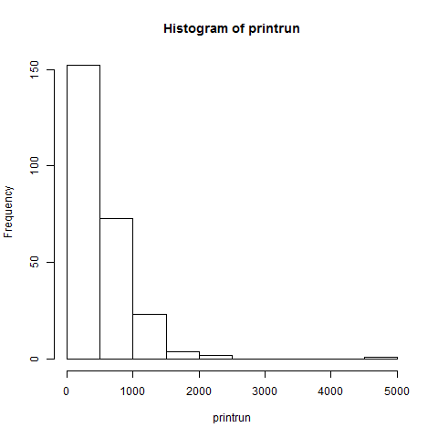
To illustrate how easy it is in R, let's turn again to Eric White's compilation of known print runs of fifteenth-century books. Here's how to make the following histogram in R:

> hist (printrun)

It really is that fast and simple.

Of course, there are a few additional steps that go into it. First, we need some data. We could put our data in a simple text file (named data.txt for this example) and open the text file. On Windows, R looks for files by default in the Documents library directory. If we only include the print runs in the text file, then R will number each row and assign a column header automatically.

To read the file into R, we need to assign it to a vector, which we'll call x:

> x <- read.table ("data.txt")

If we want to use our own column header, then we need to specify it:

> x <- read.table ("data.txt", col.names="printrun")

But my data is already a column in an Excel spreadsheet with the column header printrun, so I can just copy the column and paste it into R with the following command (on Windows) that tells R to read from the clipboard and make the first thing it finds a column header rather than data:

> x <- read.table ("clipboard", header=TRUE)

To see what's now in x, you just need to type

> x

and the whole thing will be printed out on screen. We can now access the print runs by referring to that column as x$printrun, but it might simplify the process by telling R to keep the table and its variables - its column headers, in other words - in mind:

> attach (x)

At this point, we can start playing with histograms by issuing the command hist (printrun) as above. To see all our options, we can get the help page by typing

> ?hist

The first histogram is nice, but I would really like to have solid blue bars outlined in black:

> hist (printrun, col="blue", border="black")

The hist() command uses an algorithm to determine sensible bin widths, or how wide each column is. But 500 seems too wide to me, so let's specify something else.  If I want bin widths of 250, I could specify the number of breaks as twenty:

> hist (printrun, col="blue",border="black", breaks=20)

Last time, I used bin widths of 135 and found a bimodal distribution. To do that again, I'll need to specify a range of 0 to 5130 (which is 38 * 135):

> hist (printrun, col="blue",border="black", breaks=seq (0, 5130, by=135))

To generate all the images for this post, I told R to output PNG files (it also can do TIFFs, JPGs, BMPs, PDFs, and other file types, including print-quality high resolution images, and there are also label and formatting options that I haven't mentioned here).

> png ()
> hist (printrun)
> hist (printrun, col="blue", border="black")
> hist (printrun, col="blue",border="black", breaks=20)
> hist (printrun, col="blue",border="black", breaks=seq (0, 5130, by=135))
> dev.off ()

It's as simple as that. Putting high-powered tools for statistical analysis into the hands of humanities faculty. What could possibly go wrong?

* * *

I have a few more posts about using R, but it may be a few weeks before the next one, as I'll be traveling for two conferences in the next several weeks. Next time, I'll start using R to retrace the steps of Quentin L. Burrell's article, "Some Comments on 'The Estimation of Lost Multi-Copy Documents: A New Type of Informetrics Theory' by Egghe and Proot," Journal of Informetrics 2 (January 2008): 101–5. It's an important article, and R can help us translate it from the language of statistics into the language of the humanities.