Let's learn R: Burrell on the binomial distribution

With this post, we'll start using R to retrace the steps of Quentin L. Burrell's article, "Some Comments on 'The Estimation of Lost Multi-Copy Documents: A New Type of Informetrics Theory' by Egghe and Proot," and translate it from the language of statistics into the language of the humanities.

Burrell's first important point (102) is:

A binomial distribution Bin(n, θ) with n large and θ small can be approximated by a Poisson distribution with mean λ = nθ. 

What does this mean, and why does it matter?

Burrell is responding to Proot and Egghe's formula for estimating lost editions, and they use a formula for the binomial distribution as their basis for their work. Burrell is restating a basic fact from statistics: For a data set where the number of attempts at success is large and the chance of success is small, the data will tend to fit not only a binomial distribution but also a Poisson distribution, which has some useful features for the kind of analysis he will be doing later. Where a binomial distribution has two parameters, the number of trials and the chance of success (n and θ, respectively), a Poisson distribution has only one parameter, its mean (or λ).

Is n large? In this case, yes, since n is the number of copies of each Jesuit play program that were printed. Although n isn't the same for every play program, it's a safe assumption that it's at least 150 or more, so the difference in print runs ends up not making much difference (as Proot and Egghe show in their article).

Is θ small? In this case, yes, since θ represents the likelihood of a copy to survive. With at most 5 copies of each edition surviving, θ is probably no higher than somewhere in the neighborhood of .02, and much lower for editions for fewer or no surviving copies.

So in these circumstances, can we approximate a binomial distribution with a Poisson distribution? Let's use R to illustrate how it works.

One thing that R makes quite easy is generating random data that follows a particular distribution. Let's start with 3500 observations (or, we might say, editions originally printed), with 250 trials in each (or copies of each edition that might survive) and a very low probability that any particular copy will survive, or .002. In R, we can simulate this as

> x <- rbinom (3500, 250, .002)

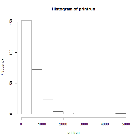
In other words, fill up the vector x with 3500 random points that follow a binomial distribution. What does it look like?

> hist (x) 

Now let's compare random points that follow Poisson distribution. We want 3500 data points again, and we also need to provide a value for λ. Since we want to see if λ really is equal to nθ, we'll use 250*.002 or .5 for λ.

> y <- rpois (3500,.5)

Let's see what the result looks like:

> hist (y)

If you look very closely, you can see that the histograms are very similar but not quite identical - which you would expect for 3500 points chosen at random.

Our data sets only have whole-number values, so let's make the histograms reflect that:

> hist (x, breaks=c(0,1,2,3,4,5))

> hist (y, breaks=c(0,1,2,3,4,5))

Let's compare the two sets of values to see how close they are. Whenever we create a histogram, R automatically creates some information about that histogram. Let's access it:

> xinfo <- hist (x, breaks=c(0,1,2,3,4,5))
> yinfo <- hist (y, breaks=c(0,1,2,3,4,5))

Typing xinfo results in a lot of useful information, but we specifically want the counts. We could type xinfo$counts, but we want to view our data in a nice table. So let's try this:

> table <- data.frame (xinfo$counts, yinfo$counts, row.names=c(0,1,2,3,4))

(We gave the table the row names of 0-4, because otherwise the row name for zero observations would be "1," and the row name for one observation would be "2," and so on, which would be confusing.) Typing table results in this:

  xinfo.counts yinfo.counts
0         3204         3208
1          252          245
2           37           41
3            6            5
4            1            1

So there you have it. For the material Proot and Egghe are dealing with, a Poisson distribution will work as well as a binomial distribution. Next time: truncated distributions, or what happens when you don't know how many editions you have to begin with.

Let's learn R: histograms for the humanities

To avoid all misunderstanding, let me make two things completely clear at the beginning: I don't know statistics and I don't know R. I did a math minor as an undergraduate, and I like to experiment with software that looks like it might be useful. That's all. Comments and corrections are welcome.

But it's been clear to me for some time that several research problems in the humanities have statistical implications, or could be productively addressed through statistical methods, and the gradually rising profile of the digital humanities will likely make statistical methods increasingly useful.

Estimating the number of lost incunable editions is one example of a research problem that required statistical expertise. For that, Paul Needham and I partnered with Frank McIntyre, an econometrician now at Rutgers. But I can't bug Frank every time I have a statistics question. He actually has to work in his own field now and again. Even when we're working on a project together, I need to understand his part enough to ask intelligent questions about it, but I haven't been able to retrace his steps, or the steps of any other statistician.

This is where R comes in. R is a free and open source statistical software package with a thriving developer community. I've barely scratched the surface of it, but I can already see that R makes some things very easy that are difficult without it.

Like histograms. Histograms are simply graphs of how many items fit into some numerical category. If you have a long list of books and the years they were printed, how many were printed in the 1460s, 1470s, or 1480s? Histograms represent data in a way that is easy to grasp. If you've ever tried it, however, you know that histograms are a huge pain to make in Excel (and real statisticians complain about the result in any case).

To illustrate how easy it is in R, let's turn again to Eric White's compilation of known print runs of fifteenth-century books. Here's how to make the following histogram in R:

> hist (printrun)

It really is that fast and simple.

Of course, there are a few additional steps that go into it. First, we need some data. We could put our data in a simple text file (named data.txt for this example) and open the text file. On Windows, R looks for files by default in the Documents library directory. If we only include the print runs in the text file, then R will number each row and assign a column header automatically.

To read the file into R, we need to assign it to a vector, which we'll call x:

> x <- read.table ("data.txt")

If we want to use our own column header, then we need to specify it:

> x <- read.table ("data.txt", col.names="printrun")

But my data is already a column in an Excel spreadsheet with the column header printrun, so I can just copy the column and paste it into R with the following command (on Windows) that tells R to read from the clipboard and make the first thing it finds a column header rather than data:

> x <- read.table ("clipboard", header=TRUE)

To see what's now in x, you just need to type

> x

and the whole thing will be printed out on screen. We can now access the print runs by referring to that column as x$printrun, but it might simplify the process by telling R to keep the table and its variables - its column headers, in other words - in mind:

> attach (x)

At this point, we can start playing with histograms by issuing the command hist (printrun) as above. To see all our options, we can get the help page by typing

> ?hist

The first histogram is nice, but I would really like to have solid blue bars outlined in black:

> hist (printrun, col="blue", border="black")

The hist() command uses an algorithm to determine sensible bin widths, or how wide each column is. But 500 seems too wide to me, so let's specify something else.  If I want bin widths of 250, I could specify the number of breaks as twenty:

> hist (printrun, col="blue",border="black", breaks=20)

Last time, I used bin widths of 135 and found a bimodal distribution. To do that again, I'll need to specify a range of 0 to 5130 (which is 38 * 135):

> hist (printrun, col="blue",border="black", breaks=seq (0, 5130, by=135))

To generate all the images for this post, I told R to output PNG files (it also can do TIFFs, JPGs, BMPs, PDFs, and other file types, including print-quality high resolution images, and there are also label and formatting options that I haven't mentioned here).

> png ()
> hist (printrun)
> hist (printrun, col="blue", border="black")
> hist (printrun, col="blue",border="black", breaks=20)
> hist (printrun, col="blue",border="black", breaks=seq (0, 5130, by=135))
> dev.off ()

It's as simple as that. Putting high-powered tools for statistical analysis into the hands of humanities faculty. What could possibly go wrong?

* * *

I have a few more posts about using R, but it may be a few weeks before the next one, as I'll be traveling for two conferences in the next several weeks. Next time, I'll start using R to retrace the steps of Quentin L. Burrell's article, "Some Comments on 'The Estimation of Lost Multi-Copy Documents: A New Type of Informetrics Theory' by Egghe and Proot," Journal of Informetrics 2 (January 2008): 101–5. It's an important article, and R can help us translate it from the language of statistics into the language of the humanities.

Abstract: "Bibliographic databases and early printing: Questions we can’t answer and questions we can’t ask"

For the upcoming meeting of the Wolfenbütteler Arbeitskreises für Bibliotheks-, Buch- und Mediengeschichte on the topic of book history and digital humanities, the paper I'm giving will briefly summarize the paper I gave at the "Lost Books" conference in June, then look specifically at the bibliographical databases of early printing that we have today. These databases are invaluable, but their current design makes some kinds of research easy and other kinds quite difficult. Along with charts and graphs, my presentation will look at some specific examples of what can and can't be done at the moment, and offer some suggestions of what might be done in the future.

Abstract: Bibliographic databases and early printing: Questions we can’t answer and questions we can’t ask.
In 1932, Ernst Consentius first proposed addressing the question of how many incunable editions have been lost by graphing the number of editions preserved in a few copies or just one and projecting an estimate based on that graph. The problem Consentius posed is in fact only a variation of a problem that can be found in many academic fields, known in English since 1943 as the “unseen species problem,” although it has not been recognized as such until very recently. Using the well-established statistical methods and tools for approaching the unseen species problem, I and Frank McIntyre have recently updated the estimate that we first published in 2010. Depending on the assumptions used, our new estimate is that between 33% (of all editions) and 49% (of codex editions, plus an indeterminate but large number of broadsides) have been lost.

The problem of estimating lost editions exemplifies how data-drive approaches can support book history, but it also illustrates how databases of early printing impose limits on research in the way they structure their records and in the user interfaces by which they make data available. Of the current database projects relevant for early printing in Germany (GW, ISTC, VD16, VD17, and USTC), each has particular advantages in the kinds of data it offers, but also particular disadvantages in how it permits that data to be searched and accessed. Clarity and consistency of formatting would help in some cases. All of the databases could profit by adding information that only one or none of the databases currently provide, such as leaf counts. User interfaces should reveal more of each database’s fields, rather than making them only implicitly visible through search results. Monolithic imprint lines, particularly those that make use of arcane or archaic terminology, must be replaced by explicit differentiation of printers and publishers.

Of the current databases, the technological advantages of VD16 are often overlooked.  Its links from editions to a separate listing of shelf marks makes it possible to count copies more simply and accurately than any other database, and its links from authors’ names to an external authority file of biographical data provide the basis for characterizing the development of printing in the sixteenth century.  Most importantly, VD16 provides open access to its MARC-formatted records, allowing an unequaled ease and accuracy when analyzing records of sixteenth-century printing. Many VD16 records lack information about such basic information as their language, however.

The missing language fields in VD16 provide an example of the challenges faced in attempting to compare bibliographic data across borders or centuries. One approach to this problem, taken by the USTC as a database of databases, is to offer relatively sparse data to users. I suggest as an alternative to this a different approach: Databases should open their data to contributions from and analysis by scholars all over the world by making their records freely available. Doing so will allow scholars of book history to pursue data-driven approaches to questions in our field.