But it's been clear to me for some time that several research problems in the humanities have statistical implications, or could be productively addressed through statistical methods, and the gradually rising profile of the digital humanities will likely make statistical methods increasingly useful.
Estimating the number of lost incunable editions is one example of a research problem that required statistical expertise. For that, Paul Needham and I partnered with Frank McIntyre, an econometrician now at Rutgers. But I can't bug Frank every time I have a statistics question. He actually has to work in his own field now and again. Even when we're working on a project together, I need to understand his part enough to ask intelligent questions about it, but I haven't been able to retrace his steps, or the steps of any other statistician.
This is where R comes in. R is a free and open source statistical software package with a thriving developer community. I've barely scratched the surface of it, but I can already see that R makes some things very easy that are difficult without it.
Like histograms. Histograms are simply graphs of how many items fit into some numerical category. If you have a long list of books and the years they were printed, how many were printed in the 1460s, 1470s, or 1480s? Histograms represent data in a way that is easy to grasp. If you've ever tried it, however, you know that histograms are a huge pain to make in Excel (and real statisticians complain about the result in any case).
To illustrate how easy it is in R, let's turn again to Eric White's compilation of known print runs of fifteenth-century books. Here's how to make the following histogram in R:
> hist (printrun)
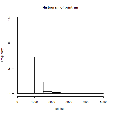
It really is that fast and simple.
Of course, there are a few additional steps that go into it. First, we need some data. We could put our data in a simple text file (named data.txt for this example) and open the text file. On Windows, R looks for files by default in the Documents library directory. If we only include the print runs in the text file, then R will number each row and assign a column header automatically.
To read the file into R, we need to assign it to a vector, which we'll call x:
> x <- read.table ("data.txt")
If we want to use our own column header, then we need to specify it:
> x <- read.table ("data.txt", col.names="printrun")
But my data is already a column in an Excel spreadsheet with the column header printrun, so I can just copy the column and paste it into R with the following command (on Windows) that tells R to read from the clipboard and make the first thing it finds a column header rather than data:
> x <- read.table ("clipboard", header=TRUE)
To see what's now in x, you just need to type
> x
and the whole thing will be printed out on screen. We can now access the print runs by referring to that column as x$printrun, but it might simplify the process by telling R to keep the table and its variables - its column headers, in other words - in mind:
> attach (x)
At this point, we can start playing with histograms by issuing the command hist (printrun) as above. To see all our options, we can get the help page by typing
> ?hist
The first histogram is nice, but I would really like to have solid blue bars outlined in black:
> hist (printrun, col="blue", border="black")

The hist() command uses an algorithm to determine sensible bin widths, or how wide each column is. But 500 seems too wide to me, so let's specify something else. If I want bin widths of 250, I could specify the number of breaks as twenty:
> hist (printrun, col="blue",border="black", breaks=20)

Last time, I used bin widths of 135 and found a bimodal distribution. To do that again, I'll need to specify a range of 0 to 5130 (which is 38 * 135):
> hist (printrun, col="blue",border="black", breaks=seq (0, 5130, by=135))

To generate all the images for this post, I told R to output PNG files (it also can do TIFFs, JPGs, BMPs, PDFs, and other file types, including print-quality high resolution images, and there are also label and formatting options that I haven't mentioned here).
> png ()
> hist (printrun)
> hist (printrun, col="blue", border="black")
> hist (printrun, col="blue",border="black", breaks=20)
> hist (printrun, col="blue",border="black", breaks=seq (0, 5130, by=135))
> dev.off ()
It's as simple as that. Putting high-powered tools for statistical analysis into the hands of humanities faculty. What could possibly go wrong?
* * *
I have a few more posts about using R, but it may be a few weeks before the next one, as I'll be traveling for two conferences in the next several weeks. Next time, I'll start using R to retrace the steps of Quentin L. Burrell's article, "Some Comments on 'The Estimation of Lost Multi-Copy Documents: A New Type of Informetrics Theory' by Egghe and Proot," Journal of Informetrics 2 (January 2008): 101–5. It's an important article, and R can help us translate it from the language of statistics into the language of the humanities.
No comments:
Post a Comment